5+2[1] 7In this first section, we are going to start from the ground up and start to familiarize ourselves with the way R works and what it expects from us. We will begin with the most basic building blocks of R data and work our way up to the data frame—the object that will be most relevant for us. While you won’t generally need to build data frames from scratch within R for your own research, it’s a good way to familiarize yourself with the structure of data in R. While we will start here with a rather simple data frame, all the principles you learn here will scale up as we start to work with much larger and more complex data frames.
I’m writing this mini-book in a language called Quarto, which allows us to carry out a bunch of neat formatting tasks with little effort. One of the big perks is that Quarto can read and process R code, so I will show you all my R code here, and you will be able to directly view the output. If you want to follow along with your own script on your personal device, you should copy and paste the commands from this document and run them locally.
First, we will start by exploring some of the basic characteristics of R.
R can be used as a simple calculator and will process both numbers and conventional mathematical operator symbols. You can run the commands below by placing your cursor at the beginning or end of the line in your script file and pressing CTRL+Enter (Windows) or Command+Return (Mac)
5+2[1] 7You should see the result displayed in the console below.
R is especially helpful for allowing us to create and store objects that we can call and manipulate later. We can create names for these objects and then use R’s ‘assignment operator,’ the <- symbol, to assign a value to our specified object name. Here, we’ll assign the previous calculation to an object that we are calling our_object.
If you run this command on your own device, you should see our_object populate in the upper-right Environment window. This is where you can find all of the objects that you create in your R session. We can run the object itself, as well as combine it with other operations
our_object <- 5+2There are some more baroque ways around this, but it’s best to operate under the impression that object names cannot include spaces (or start with numbers). This kind of thing is common in some programming languages, so there are a couple stylistic conventions to address this. I tend to use what’s called ‘snake case,’ which involves replacing spaces with underscores. There’s also ‘camel case,’ where each word has the first letter capitalized, e.g. MyVariableName. I would settle on one that you like and be consistent with it.
our_object[1] 7our_object + 3[1] 10our_object * 100[1] 700R is also useful for its implementation of functions, which you can think of in the sense you likely learned in your math classes. Functions are defined procedures that take some input value, transform that value according to the procedure, and then output a new value.
R comes with a great deal of already defined functions, and we can use these to perform all sorts of helpful operations. You can call a function by indicating it’s common name and then placing it’s required inputs between parentheses, e.g. function_name(input).Note that function inputs are also often referred to as ‘arguments’. We’ll get a lot of mileage out of functions, and part of the initial learning curve of R will be related to getting used to the range of available functions and the syntax you must follow to call them.
Now, let’s take a step back and think about some of our basic building blocks in R.
You can think of vectors as ordered sets of values. We can use the c() function (short for ‘combine’) to create a vector made up of the values we provide. Let’s make a few different vectors—each one will have 5 separate items in it, and we separate those items with commas. Note that when we want R to process something as text (and not a named object, number, or function), we put it in quotation marks.
num_vec <- c(1.2, 3.4, 5.6, 7.1, 2.8)

character_vec <- c("east", "west", "south", "south", "north")

logical_vec <- c(TRUE, FALSE, TRUE, FALSE, FALSE)
Let’s talk a bit about what we have here. Each of these vectors represents a data type in R, or, in other words, one of the basic ways in which R stores data. There are some more data types out there, but these are the most most relevant for us.
Numeric Data: As the name suggests, this is the typical fashion in which numbers are stored in R. Numeric data encompasses both continuous values and discrete values. These are essentially numbers that can have decimal places vs. integers (whole numbers).
Character Data: Character here refers to the idea of character strings. This is typically how R stores text data—as distinct strings of text. Note that, while numbers are typically processed as numeric by R, numbers can also become character data if you place them between quotation marks.
Logical Data: In R syntax, upper-case ‘true’ and ‘false’ have fixed values and, when used without quotes, will refer to these pre-defined logical values. We probably won’t use this data type much for analyses, but we will run into them in other places. They can be useful for sorting and searching through subsets of data, and we will also use logical values to turn certain procedures on or off in some functions.
Many R functions will respond differently to different data types, so it’s important to keep these in mind when you need to troubleshoot errors.
Take the mean() function, for example. As the name implies, this function will return the arithmetic mean of a numeric vector. Let’s give it the one we just made above:
mean(num_vec)[1] 4.02(1.2+3.4+5.6+7.1+2.8)/5[1] 4.02Observe that mean() gives the same response as if we had manually calculated it. Functions can make our lives a lot easier with larger amounts of data, but always make sure you’re familiar with what’s going on under the hood of any given function.
But, what happens when we run the following command?
mean(character_vec)Warning in mean.default(character_vec): argument is not numeric or logical:
returning NA[1] NAIt doesn’t make any sense to take the mean of the cardinal directions, so it will throw a warning message. We need a variable that can be represented numerically. As we’ll see, it’s a good habit to make sure you know the data type of your variables before you begin your analysis.
Now that we’ve talked about some of these basic building blocks for data, let’s talk about putting them together.
For the most part, we will be working with data frames. These are collections of data organized in rows and columns. In data science, it’s generally preferable for data to take a particular shape wherein each row indicates a single observation, and each column represents a unique variable. This is called the ‘tidy’ data format.
Let’s use the vectors we created above to mock up a little data frame. We will imagine some variables that those vectors could represent. But first, let’s make a couple more vectors.
Let’s add a vector of participant IDs associated with imaginary people in our mock data set. In accordance with tidy data, each of our rows will then represent a unique person. The column vectors will represent the variables that we are measuring for each person. Lastly, the individual cells will represent the specific values measured for each variable.
For reasons that will become clear in the next section, we are also going to add one more character vector.
p_id_vec<-c("p1", "p2", "p3", "p4", "p5")

ordinal_vec<-c("small", "medium", "medium", "large", "medium")
Now, let’s use a function to create a data frame and store it in a new object.
We can use data.frame() for this. data.frame() expects that we will give it some vectors, which it will then organize into columns. We could just give it the vectors, and it would take the vector names as column names, e.g.:
our_df <- data.frame(p_id_vec, num_vec, character_vec, ordinal_vec, logical_vec)Or we could specify new variable names and use the = sign to associate them with the vector. We will go with this latter strategy because our current vector names do not translate well to variable names.
We’ll imagine building a small data frame of dog owners and rename our vectors accordingly.
our_df<-data.frame(
  p_id = p_id_vec,
  dog_size = ordinal_vec,
  side_of_town = character_vec,
  food_per_day = num_vec,
  has_a_labrador = logical_vec
)As a slight tangent, note that we can use line breaks to our advantage with longer strings of code. The above command is identical to the one below, but some find the line-break strategy more intuitively readable. It’s most important that your code works, so you don’t have to organize it like that, but know that’s an option
our_df <- data.frame(p_id = p_id_vec, dog_size = ordinal_vec, side_of_town = character_vec, food_per_day = num_vec, has_a_labrador = logical_vec)Now our vectors make up meaningful variables in our mock data frame.
p_id = An ID for each participant in our survey of dog ownersdog_size = Owner’s ranking of their dog’s sizeside_of_town = Which part of town the owners residefood_per_day = The amount of food each owner feeds their dog daily (in ounces)has_a_labrador = true/false indicator for whether the owner has a lab or notTake a look at our new data frame by clicking on the object in our Environment window at the upper right, or by running the command View(our_df).
Once we have created a data frame, we can refer to individual variable vectors with the $ operator in R
our_df$food_per_day[1] 1.2 3.4 5.6 7.1 2.8mean(our_df$food_per_day)[1] 4.02We can look at some basic characteristics of our variables with the summary() function. Note that it will return different information depending on the data type of the variable
summary(our_df) p_id dog_size side_of_town food_per_day
Length:5 Length:5 Length:5 Min. :1.20
Class :character Class :character Class :character 1st Qu.:2.80
Mode :character Mode :character Mode :character Median :3.40
Mean :4.02
3rd Qu.:5.60
Max. :7.10
has_a_labrador
Mode :logical
FALSE:3
TRUE :2
Let’s think about these for a second.
The summary of has_a_labrador makes sense. It’s recognized as a logical vector and tells us the number of TRUEs and FALSEs
food_per_day works as well. We’re dealing with a continuous variable that allows for decimal places, so it makes sense to take the mean and look at the range and distribution.
But how about side_of_town? What that summary tells us is that this variable is a character type (or class). ‘Length’ refers to the size of the vector. So, a vector containing 5 items would be a vector of length 5. But does it make sense for us to treat the side_of_town variable as 5 totally separate strings of characters?
summary(our_df$side_of_town) Length Class Mode
5 character character Not quite. When we have two entries of “south”, for example, we want those responses to be grouped together and not treated as unique entries.
our_df$side_of_town[1] "east" "west" "south" "south" "north"For this, we will want another key R data type.
Factors are often the best way to treat categorical variables (nominal or ordinal) in R. Factors are a certain kind of vector that can only contain a number of pre-defined values. Each of these pre-defined values is considered a ‘level’ of the factor. So, we want side_of_town to be a factor variable with 4 levels: east, west, south, and north.
We can turn this variable into a factor with R’s as.factor() function.
our_df$side_of_town <- as.factor(our_df$side_of_town)Check the summary() output again and notice how the output is reported now. Instead of simply listing that the vector contained 5 character strings, we can now see the different levels and the number of people who belong to each side of town.
summary(our_df) p_id dog_size side_of_town food_per_day
Length:5 Length:5 east :1 Min. :1.20
Class :character Class :character north:1 1st Qu.:2.80
Mode :character Mode :character south:2 Median :3.40
west :1 Mean :4.02
3rd Qu.:5.60
Max. :7.10
has_a_labrador
Mode :logical
FALSE:3
TRUE :2
Now, let’s think about dog_size. This should clearly be a factor variable as well. But, unlike food_per_day, the levels of this variable have an apparent order, from small to large.
The factor() function allows us to turn a vector into a factor, as well as manually specify the levels. Additionally, we can activate a process in the function letting it know that we want the order to matter.
our_df$dog_size <- factor(
  our_df$dog_size,
  levels=c("small", "medium", "large"),
  ordered = TRUE
  )
Take a look back at the summary. Now, instead of 5 separate character strings, we can see the breakdown of how many people have a dog of a certain size.
summary(our_df) p_id dog_size side_of_town food_per_day has_a_labrador
Length:5 small :1 east :1 Min. :1.20 Mode :logical
Class :character medium:3 north:1 1st Qu.:2.80 FALSE:3
Mode :character large :1 south:2 Median :3.40 TRUE :2
west :1 Mean :4.02
3rd Qu.:5.60
Max. :7.10 Note that the str() command is also useful for quickly gleaning the various data types of variable columns within a data frame. It will show us our variable names, the data types, and then a preview of the first several values in each variable column.
We can also verify that dog_size has been successfully re-coded as an ordered factor.
str(our_df)'data.frame': 5 obs. of 5 variables:
$ p_id : chr "p1" "p2" "p3" "p4" ...
$ dog_size : Ord.factor w/ 3 levels "small"<"medium"<..: 1 2 2 3 2
$ side_of_town : Factor w/ 4 levels "east","north",..: 1 4 3 3 2
$ food_per_day : num 1.2 3.4 5.6 7.1 2.8
$ has_a_labrador: logi TRUE FALSE TRUE FALSE FALSEThere are cases where you will want to convert a column like p_id to a factor variable as well, but often we just need a variable like p_id to serve as a searchable index for individual observations, so we can leave it be for now.
This is all part of the process of data cleaning, where we make sure our data is structured in a fashion that’s amenable to analysis. This re-coding of variables is an essential component, and we’ll see plenty more tasks in this vein when we work with GSS data later on.
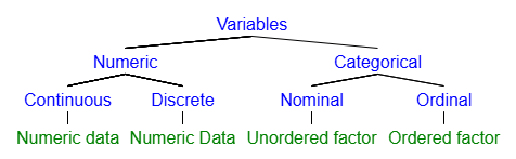
As we close this section, here is a figure to help you internalize the hierarchy of variable types based on the levels of measurement. The bottom level of the hierarchy (in green) reflects the R data type that is best aligned with a particular measurement level. Also recall that numeric data can either be interval or ratio, though we will generally treat these similarly.
For our last bit, let’s learn a little about working with functions that don’t come included in base R.